ISPRS Test Project on Urban Classification and 3D Building Reconstruction: Evaluation of Object Detection Results
Franz Rottensteiner
Institute of Photogrammetry and GeoInformation, Leibniz Universität Hannover, Nienburger Str.1, 30167 Hannover, Germany; E-mail: rottensteiner@ipi.uni-hannover.de
The evaluation of object detection results is based on the method described in (Rutzinger et al., 2009). The software used for evaluation reads the reference and the object detection results, converts them into a label image and then carries out the evaluation as described in the paper. The output consists in a text file containing the evaluation results and in a few images that visualize these results.
Interpretation of the images:
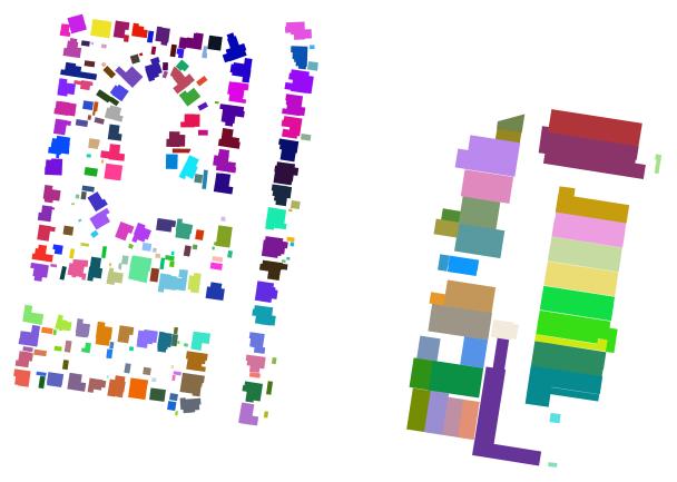
reference_labels.tif: the label
image corresponding to the reference.
Example:
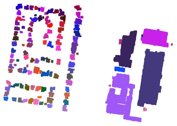
results_labels.tif: the label
image corresponding to the object detection results.
Example:
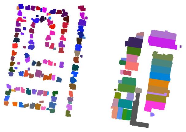
results_labels_clarified.tif: the label image
corresponding to the object detection results after topological
clarification as described in (Rutzinger et al., 2009). In this label
image, objects corresponding to multiple labels in the reference are
split up so that there only remain (1:0), (0:1), and (1:1) relations
between overlapping objects in the two data sets.
Example:
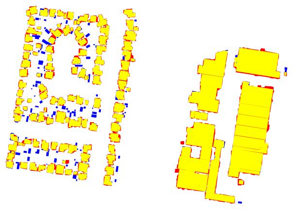
evalPix.tif: this image contains the evaluation on a per-pixel level. The meaning of the colours is:
Yellow: True positive pixels
Blue: false negative pixels
Red: false positive pixels.
Example:
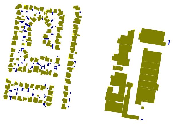
Evaluation_ReferenceObjects_Class.tif: this image contains the evaluation on a per-object level from the point of view of the reference data. The meaning of the colours is:
Ochre: True positive pixels in reference objects classified as true positives
Yellow: False negative pixels in reference objects classified as true positives
Dark blue: False negative pixels in reference objects classified as false negatives
Bright blue: True positive pixels in reference objects classified as false negatives.
Example:
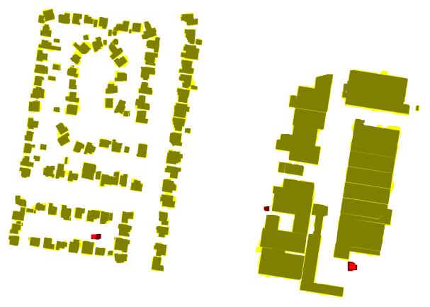
Evaluation_ExtractedObjects_Class.tif: this image contains the evaluation on a per-object level from the point of view of the topologically clarified object detection results. The meaning of the colours is:
Ochre: True positive pixels in extracted objects classified as true positives
Yellow: False positive pixels in extracted objects classified as true positives
Dark red: False positive pixels in extracted objects classified as false positives
Bright red: True positive pixels in extracted objects classified as false positives.
Example:
Interpretation of the evaluation results contained in the text file:
At the beginning, the number of objects found in the detection results and the reference, respectively, before topological clarification are reported. Only objects larger than a specified threshold will be considered for evaluation. In the example below, only objects larger than 2.5 m2 are considered.
Evaluation of object detection results
======================================
Number of objects in the reference: 235 ( 235 larger than 2.5 m^2).
Number of objects detected: 116 ( 116 larger than 2.5 m^2).
This is followed by a listing of the thresholds used for classifying the overlap between objects in the two data sets. There are four categories of overlap (none / weak / partial / strong), based on the percentage of the area of an object that is covered by the corresponding object in the other data set. Note that this classification is not symmetric. Details about how the overlap is determined can be found in (Rutzinger et al., 2009) and (Rottensteiner et al., 2005). Note that in the object-based classification, all objects having an overlap larger than the threshold “weak vs. partial” (50% in the example below) with objects in the other data set are counted as true positives.
Thresholds for overlap criterion:
=================================
None vs Weak [%]: 10.0
Weak vs Partial [%]: 50.0
Partial vs Strong [%]: 80.0
The
geometrical accuracy of the boundary polygons for corresponding
objects is evaluated next. For each vertex of an extracted polygon,
the nearest point on the boundary of the corresponding object in the
reference is searched. This point does not necessarily correspond to
a vertex of that polygon. The (2D) Euclidean distance d
between the corresponding points is found. If this distance is larger
than a threshold
(3 m in the example below), it is discarded.
Finally, the RMS error of the distances RMSd
is computed:

A similar procedure is applied to the centres of gravity of corresponding objects. However, for the centres of gravity, both the RMS errors in x and y are reported, i.e.,
 and
and

In both cases, N is the number of points for which a correspondence has been found within a predefined search buffer. Furthermore, all these RMS errors are determined in both directions. Where the numbers are given for or “extracted boundaries”, the nearest point on the reference boundary was determined for each boundary polygon vertex in the extraction results. In the example below, there were 1413 boundary points in the extraction results, of which 1329 were found to have a correspondence (within 3 m) in the reference. Where the numbers are given for or “reference boundaries”, the nearest point on an extracted boundary was searched for each reference polygon vertex. In the example below, there were 6185 boundary points in the reference, of which 2349 were found to have a correspondence (within 3 m) in the extraction results. (Note that this small number is due to a large number of small objects that were not correctly detected).
Evaluation of Geometrical Accuracy:
===================================
Distance threshold: 3.0 [m]
Total RMS of extracted boundaries: 0.98 [m] (determined from 1329 of 1413 possible correspondences)
Total RMS of centres of gravity of extracted objects (X / Y): 0.58 [m] /0.54 [m] (determined from 103 of 115 possible correspondences)
Total RMS of reference boundaries: 1.08 [m] (determined from 2349 of 6185 possible correspondences)
Total RMS of centres of gravity of reference objects (X / Y): 0.58 [m] /0.54 [m] (determined from 103 of 153 possible correspondences)
Histograms are given for the RMSd errors of the boundary polygons. Each histogram entry gives the number of boundary polygons for which the RMSd (computed only for the points of that polygon) was in the respective bin.
Histogram of RMS of extracted boundaries, 0.05, 0.15, 0.25, 0.35, 0.45, …
, 2, 0, 1, 4, 5, …
Histogram of RMS of reference boundaries, 0.05, 0.15, 0.25, 0.35, 0.45, …
, 0, 0, 0, 0, 2, …
Topological clarification is carried out next. Originally, there may be (1:0), (0:1), (1:1), (1:M), (M:1), or (M:N) relations between objects in the reference and objects. The number of instances of (1:M), (M:1), or (M:N) relations are reported along with the object identifiers between which they occur (note that the object identifier is encoded in the green band of the label images). For instance, in the example below, there are zero 1:M relations, 13 M:1 relations, and two M:N relations. The first M:1 relation occurs between the extracted object 1 and two reference objects (33 and 34). The first M:N relation involves reference objects 52 and 53, which overlap with the objects 33 and 42 in the extraction results. Topological clarification involves changing the label image corresponding to the extraction results so that in the end there are no more (1:M), (M:1), or (M:N) relations, carried out in the way described in (Rutzinger et al., 2009). The number of objects in the detection results after the clarification is given, too.
Topological clarification of object extraction results:
=======================================================
Objects with a correspondence of 1 : M (reference : results): 0
Objects with a correspondence of M : 1 (reference : results): 13
Results: 1; Reference: 33 / 34
Results: 8; Reference: 3 / 22
Results: 19; Reference: 74 / 166
Results: 35; Reference: 13 / 176
Results: 49; Reference: 228 / 133
Results: 51; Reference: 15 / 42
Results: 57; Reference: 138 / 222 / 221 / 220 / 219 / 158 / 157 / 139 / 233
Results: 76; Reference: 152 / 153
Results: 87; Reference: 51 / 145 / 150 / 149 / 148 / 147 / 146 / 141 / 144 / 143 / 142 / 151 / 234
Results: 90; Reference: 232 / 216 / 124
Results: 97; Reference: 111 / 112
Results:100; Reference: 95 / 94
Results:102; Reference: 116 / 117
Object tuples with a correspondence of M : N (reference : results): 2
Reference: 52 / 53; Results : 33 / 42
Reference: 136 / 155 / 154 / 156 / 137 / 140 / 135 / 134; Results : 36 / 46
--------------------------------------------------------------------------
--------------------------------------------------------------------------
Number of detected objects after topological clarification: 154
--------------------------------------------------------------------------
--------------------------------------------------------------------------
This is followed by a histogram of the area overlap of objects, given both for the reference and for the extraction result. Any entry in the histogram is the number of objects for which the percentage of their areas covered by objects in the other data sets corresponds to the respective bin.
Histogram of overlap of reference objects
=========================================
Histogram of overlap of reference objects, 2.5, 7.5, 12.5, 17.5, 22.5, …
, 82, 0, 0, 0, 0, …
Histogram of overlap of detected objects
========================================
Histogram of overlap of detected objects, 2.5, 7.5, 12.5, 17.5, 22.5, …
, 1, 0, 0, 0, 0, …
Again, these histogram can be converted into a graph easily using MS Excel:
Now, the results of the evaluation are finally reported. Evaluation is carried out on a per-area level, on a per-object level, and on a per-object level balanced by area. In all cases, the completeness, the correctness, and the quality of the results are determined:
In these equations, #TP, #FN, and #FP are the numbers of true positive, false negative, and false positive objects, respectively. First, the results of the per-area evaluation are given. Here, the numbers of pixels belonging to the categories mentioned above are counted. First, the numbers of true positive, false negative, false positive, and true negative pixels are given. After that, the evaluation indices are presented.
Evaluation on a per-area level (pixel size: 0.100 m)
=====================================================
Number of object pixels (reference): 4148433( 41484.3 m^2)
Number of object pixels (detection results): 4457800( 44578.0 m^2)
Number of true positives: 3910535( 39105.3 m^2)
Number of false positives: 547265( 5472.6 m^2)
Number of false negatives: 237898( 2379.0 m^2)
Number of true negatives: 14685502( 146855.0 m^2)
Per-area completeness: 94.3%
Per-area correctness: 87.7%
Per-area quality: 83.3%
This is followed by the evaluation on a per-object level. In this context, an object is considered to be a true positive if a certain minimum percentage of its area is covered by objects in the other data set. Note that this definition is not symmetric, so that the number of true positives is different for the two data sets. First, the numbers of true positive, false negative, false positive, and true negative objects are given. After that, the evaluation indices are presented. Firstly, they are given on a purely object-based level. Secondly, the per-object evaluation is balanced by the object area. That is, each object is weighted by its total area; an object only covered by, say, 70% would be counted with 100% of its area. Thirdly, the quality numbers are given for all objects covering an area larger than a threshold that depends on the object type. This numbers should be representative for the “most relevant” objects. For buildings and trees, the area threshold is 50 m2.
Evaluation on a per-object level (Threshold for classification as a true positive: 50.0%
=========================================================================================
Number of objects (reference): 235( 41484.3 m^2)
Number of detected objects: 154( 44578.0 m^2)
Number of true positive reference objects: 152( 39646.4 m^2)
Number of true positive detected objects: 151( 44357.0 m^2)
Number of false positives: 3( 221.0 m^2)
Number of false negatives: 83( 1837.9 m^2)
Per-object completeness: 64.7%
Per-object correctness: 98.1%
Per-object quality: 63.9%
Per-object completeness balanced by area: 95.6%
Per-object object correctness balanced by area: 99.5%
Per-object object quality balanced by area: 95.1%
Per-object completeness for objects larger than 50.0 m^2: 89.1%
Per-object correctness for objects larger than 50.0 m^2: 98.6%
Per-object quality for objects larger than 50.0 m^2: 88.0%
Finally, the object-level evaluation is carried out as a function of the object size. First, completeness, correctness, and quality are presented as a function of the object area, i.e., these percentages are determined separately for all objects belonging to the corresponding area interval. After that, cumulative histograms are given. They show the quality numbers for all objects larger than the area corresponding to the respective histogram bin.
Evaluation on a per-object level as a function of the object area:
==================================================================
Area [m^2], 12.5, 37.5, 62.5, 87.5, 112.5, 137.5, 162.5, 187.5, 212.5, 237.5,>250.0
Completeness, 3.1, 23.9, 50.0, 33.3, 100.0, 100.0, 100.0, 100.0, 100.0, 100.0, 100.0,
Correctness , , 85.7, 100.0, 75.0, 66.7, 100.0, 100.0, 100.0, 100.0, 100.0, 100.0,
Quality , , 23.0, 50.0, 30.0, 66.7, 100.0, 100.0, 100.0, 100.0, 100.0, 100.0,
Evaluation on a per-object level as a function of the object area (cumulative):
===============================================================================
Area [m^2], 12.5, 37.5, 62.5, 87.5, 112.5, 137.5, 162.5, 187.5, 212.5, 237.5,>250.0
Completeness, 64.5, 74.3, 89.1, 98.4, 100.0, 100.0, 100.0, 100.0, 100.0, 100.0, 100.0,
Correctness , 98.1, 98.1, 98.6, 98.4, 99.2, 100.0, 100.0, 100.0, 100.0, 100.0, 100.0,
Quality , 63.7, 73.2, 88.0, 96.9, 99.2, 100.0, 100.0, 100.0, 100.0, 100.0, 100.0,
Again, these histogram can be converted into a graph easily using MS Excel:
This is followed by a histogram of the areas of the objects in the reference and then by histograms of objects that were either classified as TP, FP, or FN.
Histogram of area coverage of all objects in the reference:
===========================================================
Area[m^2], 12.5, 37.5, 62.5, 87.5, 112.5, 137.5, 162.5, 187.5, 212.5, 237.5,>250.0
, 32, 46, 30, 3, 11, 20, 23, 13, 16, 6, 34,
Histogram of area coverage of true positives (reference):
=========================================================
Area[m^2], 12.5, 37.5, 62.5, 87.5, 112.5, 137.5, 162.5, 187.5, 212.5, 237.5,>250.0
, 1, 11, 15, 1, 11, 20, 23, 13, 16, 6, 34,
Histogram of area coverage of true positives (New):
===================================================
Area[m^2], 12.5, 37.5, 62.5, 87.5, 112.5, 137.5, 162.5, 187.5, 212.5, 237.5,>250.0
, 0, 6, 18, 3, 2, 6, 19, 23, 13, 18, 43,
Histogram of area coverage of false negatives:
==============================================
Area[m^2], 12.5, 37.5, 62.5, 87.5, 112.5, 137.5, 162.5, 187.5, 212.5, 237.5,>250.0
, 31, 35, 15, 2, 0, 0, 0, 0, 0, 0, 0,
Histogram of area coverage of false positives:
==============================================
Area[m^2], 12.5, 37.5, 62.5, 87.5, 112.5, 137.5, 162.5, 187.5, 212.5, 237.5,>250.0
, 0, 1, 0, 1, 1, 0, 0, 0, 0, 0, 0,
Rottensteiner, F., Trinder, J., Clode, S., Kubik, K., 2005. Using the Dempster-Shafer method for the fusion of LIDAR data and multi-spectral images for building detection. Information Fusion 6(4):283-300.
Rutzinger, M., Rottensteiner, F. Pfeifer, N., 2009. A comparison of evaluation techniques for building extraction from airborne laser scanning. IEEE Journal of Selected Topics in Applied Earth Observations and Remote Sensing 2(1):11-20.