Introduction
One of the major topics in photogrammetry is the automated extraction of urban objects from data acquired by airborne sensors. What makes this task challenging is the very heterogeneous appearance of objects like buildings, streets, trees and cars in very high-resolution data, which leads to high intra-class variance while the inter-class variance is low. Focus is on detailed 2D semantic segmentation that assigns labels to multiple object categories. Further research drivers are very high-resolution data from new sensors and advanced processing techniques that rely on increasingly mature machine learning techniques. Despite the enormous efforts spent, these tasks cannot be considered solved, yet. To our knowledge, no fully automated method for 2D object recognition is applied in practice today although at least two decades of research have tried solving this task. One major problem that is hampering scientific progress is a lack of standard data sets for evaluating object extraction, so that the outcomes of different approaches can hardly be compared experimentally. This "semantic labeling contest" of ISPRS WG III/4 is meant to resolve this issue.
To this end we provide two state-of-the-art airborne image datasets, consisting of very high resolution treue ortho photo (TOP) tiles and corresponding digital surface models (DSMs) derived from dense image matching techniques. Both areas cover urban scenes. While Vaihingen is a relatively small village with many detached buildings and small multi story buildings, Potsdam shows a typical historic city with large building blocks, narrow streets and dense settlement structure.
Each dataset has been classified manually into six most common land cover classes. We provide the classification data (label images) for approximately half of the images, while the ground truth of the remaining scenes will remain unreleased and stays with the benchmark test organizers to be used for evaluation of submitted results. Participants shall use all data with ground truth for training or internal evaluation of their method.
Six categories/classes have been defined:
- Impervious surfaces (RGB: 255, 255, 255)
- Building (RGB: 0, 0, 255)
- Low vegetation (RGB: 0, 255, 255)
- Tree (RGB: 0, 255, 0)
- Car (RGB: 255, 255, 0)
- Clutter/background (RGB: 255, 0, 0)
The clutter/background class includes water bodies (present in two images with part of a river) and other objects that look very different from everything else (e.g., containers, tennis courts, swimming pools) and that are usually not of interest in semantic object classification in urban scenes, however note that participants must submit labels for all classes (including the clutter/background class). For instance, it is not possible to submit only classification results for the category building.
Submission of results
A full classification of each patch for which we do not provide ground truth is expected. Validation of provided reference is not done and if delivered, the data will be ignored.
The naming convention for tif files containing the label information is derived from the provided files:
top_mosaic_09cm_areaXX_class.tif, where XX is the number of the patch, e.g. top_mosaic_09cm_area8_class.tif, or top_mosaic_09cm_area38_class.tif. The tif label files must have the same size as the original tile.
→ DO NOT USE ANY TIF compression format, not even lossless; INSTEAD zip all original tif-files into one zip file.
Such a zip-file containing all the resulting tif-label files is typically not larger than 10 MB. This zip-file, together with a detailed description of the method used (or reference to a published paper) should be sent to Markus Gerke. Emails with attachments larger than 15MB will not be processed.
Evaluation of results
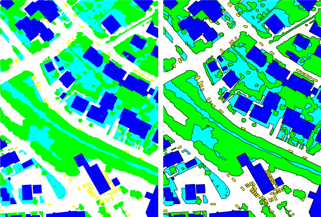
Per tile we use a reference classification which was produced in the same manner as the reference tiles we provide for training. Besides the full reference, we also prepared references where the boundaries of objects are eroded by a circular disc of 3 pixel radius. Those eroded areas are then ignored during evaluation. The motivation is to reduce the impact of uncertain border definitions on the evaluation.

Ground truth used for the assessment: "full_reference" (left), "no_boundary" (right). Black areas in the right hand reference will be ignored
The evaluation is based on the computation of pixel-based confusion matrices per tile, and an accumulated confusion matrix. From those matrices different measures are derived: per class we compute completeness (recall), correctness (precision) and F1 score (see below for details), and through the normalisation of the trace from the confusion matrix we derive an overall accuracy.
Those measures are computed twice (for full_reference and no_boundaries).
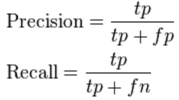
The confusion matrices are defined in a way that in row direction the reference is given, while in column direction the prediction. The cells are then normalised with respect to the reference. This means that rows add up to 100% (round-off errors might occur). The True Positive, tp, pixels are derived from the main diagonal elements, while the False Positive, fp, is computed from the sum per column, excluding the main diagonal element. Likewise, the False Negative, fn, is the sum along the row, excluding the main diagonal element. From those tp, fp, fn per object the usual measures are derived:

Precision (correctness) and recall (completeness) derived from tp, fp, fn. Source of image: Wikipedia
The F1-score is defined as the harmonic mean of precision and recall:

F1-score. Source of image: Wikipedia
The accumulated confusion matrix is simply the sum of all individual confusion matrices, where the absolute cell values are added up.
The front page of the result table contains per participant the F1 scores for the relevant classes (without clutter) and the overall accuracy, as derived from the no_boundary reference and the accumulated confusion matrix. In addition an indication is given whether the algorithm used by the participant is supervised, unsupervised, or a mixture (hybrid). The "P"-link opens a documentation/paper provided by the participant describing the used appraoch. The "D"-link (details) opens another webpage where all individual confusion matrices and derived measures (per tile, per reference set) are shown. In addition per tile a "red green" image is shown indicating areas of wrong classification.
Note that on purpose we do not provide a ranking of results. The order of appearance in the table is according to the order of result submission.
Specific data descriptions, a data request form and the result page can be reached via the left-hand pane.